Plotting Data
yt offers a lot of functionality for plotting. See how-to-make-plots
for a full discussion. However, the spatial plots are geared mainly to 3D data,
so yt_georaster provides a simple interface to making spatial plots of 2D
data. The plot() function
will plot a single field, accepting optional arguments for a center, width,
and height. If you are working in a Jupyter notebook, use p.show() to
display the plot inline.
>>> import yt
>>> import yt.extensions.georaster

>>> filenames = glob.glob("Landsat-8_sample_L2/*.TIF") + \
...   glob.glob("M2_Sentinel-2_test_data/*.jp2")
>>> ds = yt.load(*filenames)

>>> field = ("LC08_L2SP_171060_20210227_20210304_02_T1", "NDVI")
>>> p = ds.plot(field, center=ds.domain_center,
...             width=(50, "km"), height=(50, "km"))
>>> p.set_cmap(field, "RdYlGn")
>>> p.save("plot_1.png")
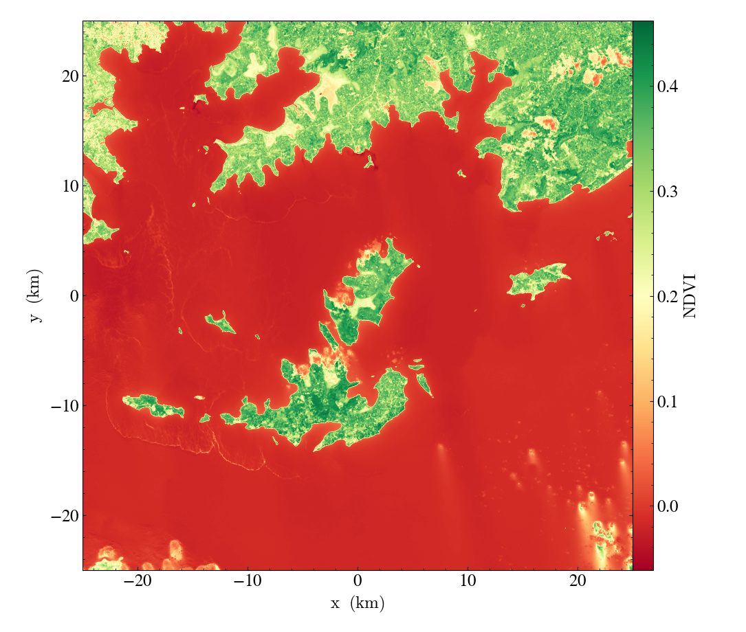
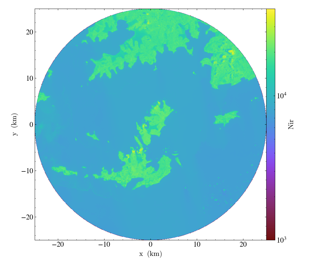
Plotting Data Containers
The plot() function also
accepts a data_source keyword to plot data only within the container. The
center, width, and heigh will be set automatically base on the container.
>>> cir = ds.circle(ds.domain_center, (25, "km"))
>>> field = ('LC08_L2SP_171060_20210227_20210304_02_T1', "nir")
>>> p = ds.plot(field, data_source=cir)
>>> p.set_zlim(field, 1000, 40000)
>>> p.set_axes_unit('km')
>>> p.save("plot_2.png")
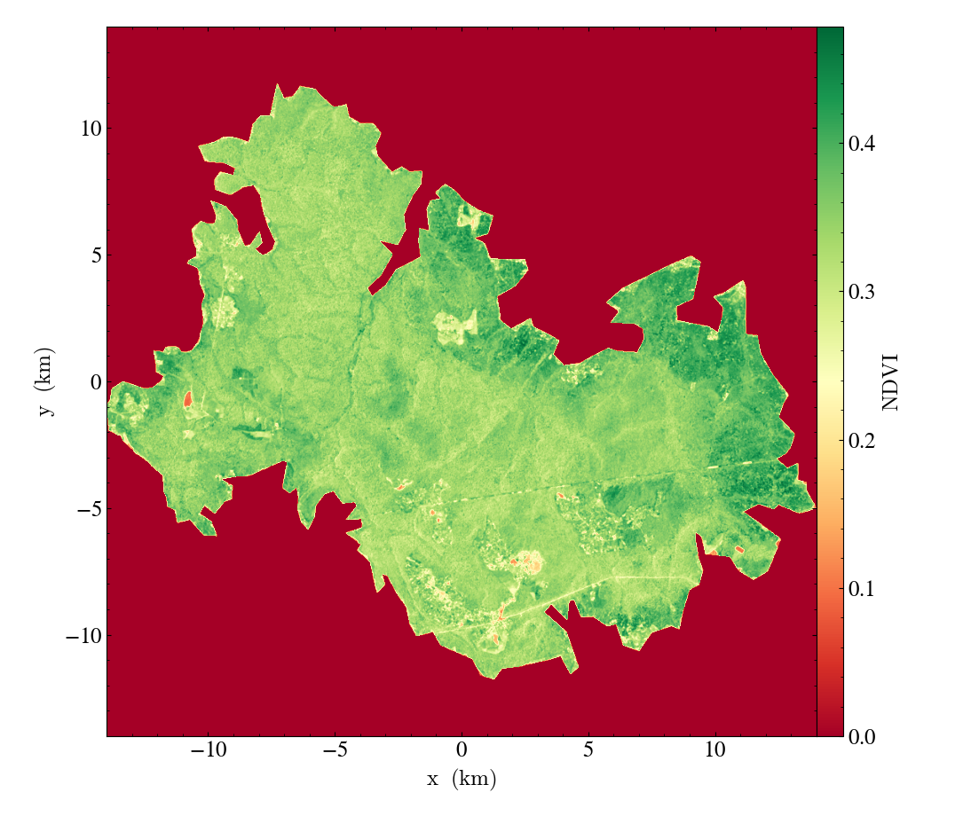
>>> poly = ds.polygon("example_polygon_mabira_forest/mabira_forest.shp")
>>> field = ("LC08_L2SP_171060_20210227_20210304_02_T1", "NDVI")
>>> p = ds.plot(field, data_source=poly)
>>> p.set_cmap(field, "RdYlGn"))
>>> p.set_axes_unit("km")
>>> p.save("plot_3.png")